Texture Paper Reading-[Let There Be Color!]

• Let There Be Color! - Large-Scale Texturing of 3D Reconstructions
  • 
  • Paper.pdf

  • In this paper we therefore present the first unified texturing approach that handles large, realistic datasets reconstructed from images with a structure-from-motion plus multi-view stereo pipeline.

  • millions of triangles within less than two hours.

  • Related
    • view selection
      • blend multiple views per face[5,13]
      • one view per face[9,10,15,23]
      • one view per texel[19]
      • one view per face but blend close to texture patch borders[2,6]
      • single view per face based on a pairwise Markov random field[15]
        • smoothness term models
      • view blend
        • weight blending[5]
          • masks indicating
          • angle to weight

          • suggest the use of vertex colors in combination with mesh subdivision

        • blending in frequency space[2,6]
      • blend pixels based on angle and proximity to the model[13]
      • view-dependent texturing— Lumigraph[4]
    • Color Adjustment
      • 
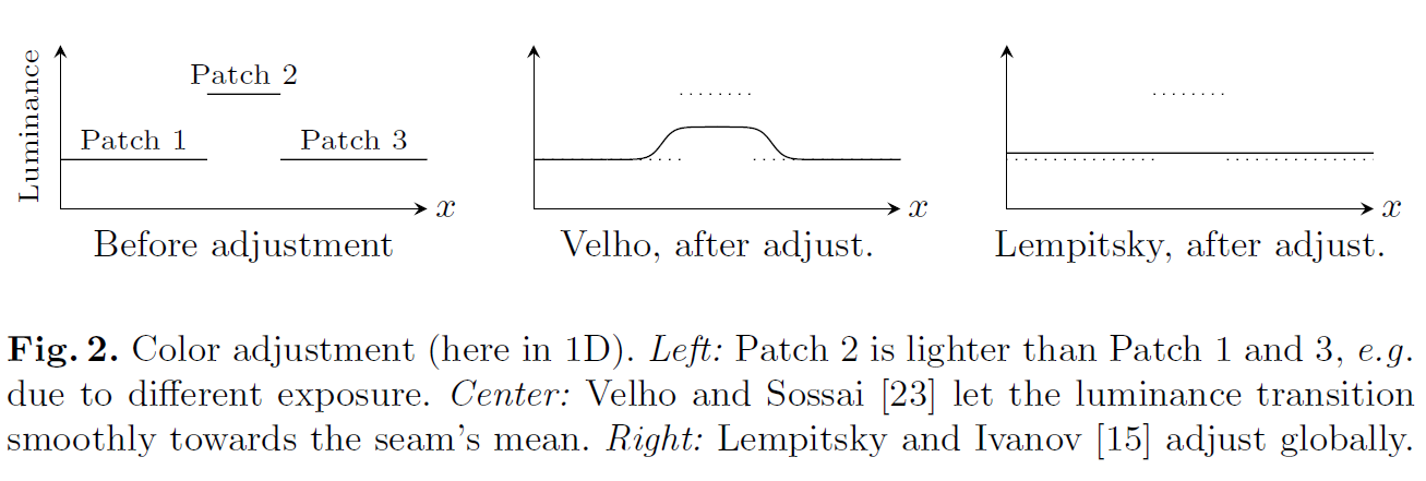
      • local
        • seam's mean[23]
          • heat diffusion
      • global
        • globally optimal luminance correction terms[15]

          • After adjustment luminance differences at seams should be small and the derivative of adjustments within a texture patch should be small

  • Assumptions and Base Method
    • Pairwise Markov random field energy formulation[15]
    • $$ \begin{aligned} E(l)&=\sum_{F_i\in Faces}E_{data}(F_i, l_i)+\sum_{F_i\in Faces}E_{smooth}(F_i, F_j, l_i, l_j)&(1) \end{aligned} $$
      • $l$: labeling of views
      • $F$: mesh face
      • $E_{data}$: good views for texturing a face

        1. base method: the angle between viewing direction and face normal.

        2. project a face into a view and use the projection’s size as data term[2]

        3. Lumigraph’s view blending weights face normal[4] 💩

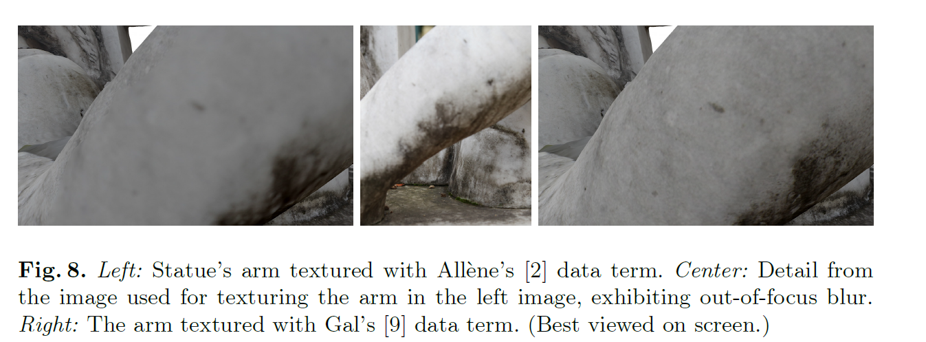
        4. the gradient magnitude of the image integrated over the face’s projection[9]

           • to solve close-up the faces closest to the camera that not be in focus and lead to a blurry texture.
           • $x,y \pm64pixel$
      • $E_{smooth}$: minimizes seam (i.e., edges between faces textured with differentimages) visibility.
      • $E(l)$minimized with graph cuts and alpha expansion[3]
    • This Paper [Compute seam color]

      • We found, that computation of the seam error integrals is a computational bottleneck and cannot be precomputed due to the prohibitively large number of combinations. Furthermore, it favors distant or low-resolution views since a blurry texture produces smaller seam errors, an issue that does not occur in their datasets.

      • Add a additive correction $g$
      • $$ \begin{aligned} &\underset{\mathbf{g}}{\argmin}\sum_v \big(f_{v_{left}} + g_{v_{left}} - (f_{v_{right}}+g_{v_{right}})\big)^2 + \frac{1}{\lambda}\sum_{v_i,v_j}(g_{v_i}-g_{v_j})^2&(2) \end{aligned} $$
        • $v$: vexel
        • $v_{left}$: vexel at left of seam
        • $v_{right}$: vexel at left of seam
        • $v_i,v_j$: vexel at same seam and adjacent
        • $f_{v*}$: color of vexel
        • $g$: additive correction

      • After fnding optimal gv for all vertices the corrections for each texel are interpolated from the $g_v$ of its surrounding vertices using barycentric coordinates.

  • Large-Scale Texturing Approach
    • Preprocessing
      • check face visibility by ColNet[11]
      • precompute the data terms for Equation $(1)$
    • View Selection
      • graph cuts and alpha expansion[3]
      • replace[9] the Data term to
        • $E_{data} = -\int_{\phi(F_i,l_i)}\Vert\nabla(I_{l_i}(p))\Vert_2dp$💩
          • $F_i$: face
          • $\phi(F_i,l_i)$: $F_i$’s projection
          • $I_{l_i}$: Sobel operator
          • $\Vert\nabla(I_{l_i})\Vert_2$: gradient magnitude
          • 大概意思就是，面投影到图片，计算投影区的Sobel operator, 如果投影区太小没有像素，就gradient magnitude at the projection's centroid and multiply it with the projection area., 最后把它们加一块
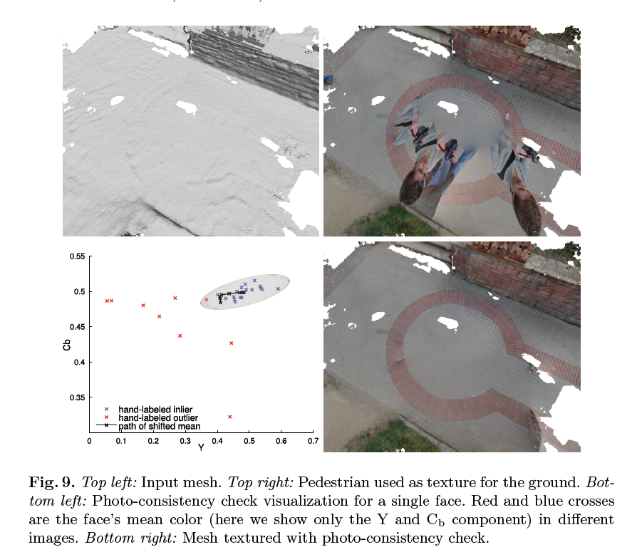
      • Photo-Consistency Check [检查遮挡和行人]

        • introduce an additional step to ensure photo-consistency of the texture.

        • assuming

          • the majority of views see the correct color.

          • A minority may see wrong colors

        • reject inconsistent views
          • mean[19]
          • median[13]
          • mean-shift algorithm[this]
            1. Compute the face projection’s mean color $c_i$ for each view $i$ in which the face is visible.
            2. Declare all views seeing the face as inliers.
            3. Compute mean $\mu$ and covariance matrix $\Sigma$ of all inliers’ mean color $c_i$.
            4. Evaluate a multi-variate Gaussian function $exp(-\frac{1}{2}(c_i-\mu)^T\Sigma^{-1}(c_i-\mu))$ each view in which the face is visible.
            5. Clear the inlier list and insert all views whose function value is above a threshold $6E-3$ as default
            6. Repeat 3.-5. for 10 iterations or until all entries of $\Sigma$ drop below $10E-5$, the inversion of $\Sigma$ becomes unstable, or the number of inliers drops below 4
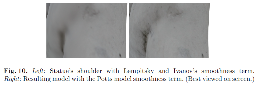
      • replace the Smoothness Term
        • based on the Potts model
        • $E_{smooth} = [l_i\neq l_j]$💩
          • $[\cdot]$: is the Iverson bracket, 满足条件就是1，不满足就是0.
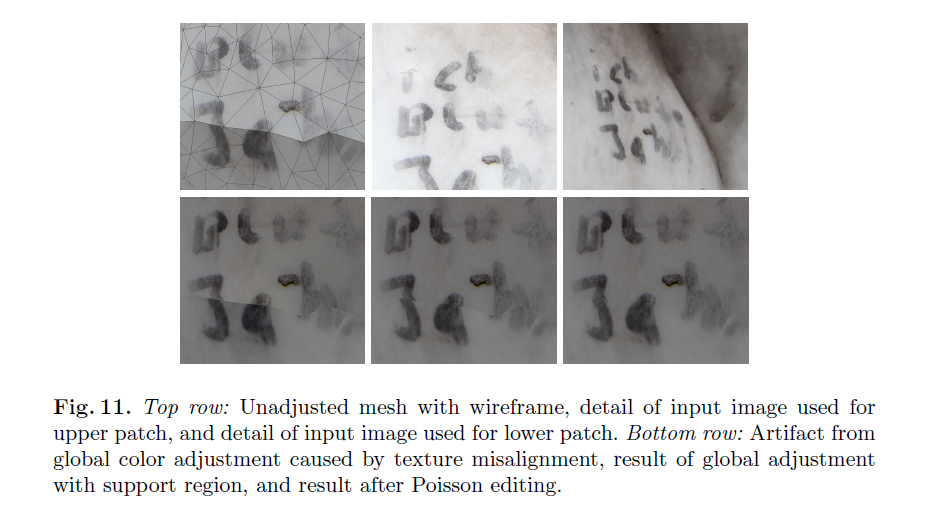
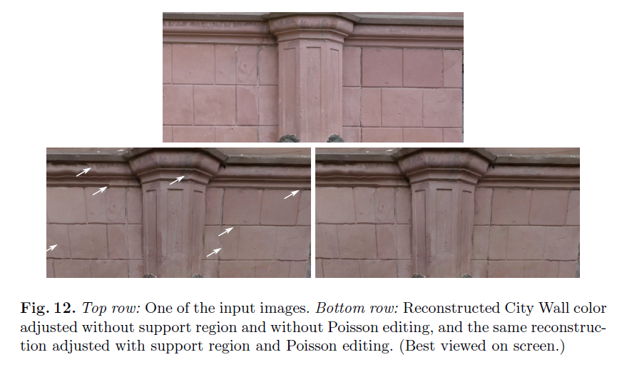
    • Color Adjustment
      • local adjustment with Poisson editing[16]
        • global adjustment[15] problem

        • the vertex v’s projection into the two images adjacent to the seam. If there are even small registration errors (which there always are), both projections do not correspond to exactly the same spot on the real object. Also, if both images have a different scale the looked up pixels span a different footprint in 3D. This may be irrelevant in controlled lab datasets, but in realistic multi-view stereo datasets the lookups from effectively different points or footprints mislead the global adjustment and produce artifacts.

      • Color Lookup Support Region
        • 
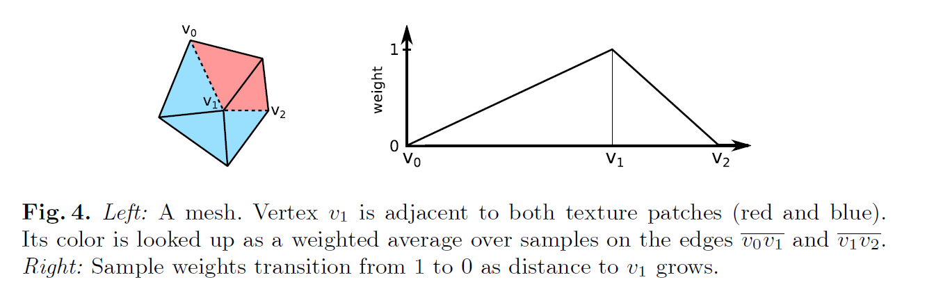
        • $v_1$点的颜色等于两条边的颜色*距离权重
        • Equation 2 matrix form
        • $$ \mathbf{\Vert Ag-f\Vert_2^2+\Vert\Gamma g\Vert_2^2=g^T(A^TA+\Gamma^T\Gamma)g-f^TAg+f^Tf} $$
          • $\mathbf{f}$: vector, stacked $f_{v_{left}} - f_{v_{right}}$
          • $\mathbf{A}$: sparse matrix with $\pm 1$
          • $\mathbf{\Gamma}$: sparse matrix with $\pm 1$
        • minimize it with conjugate gradient when $\frac{\Vert r\Vert_2}{\Vert\mathbf{A^Tf}\Vert_2}<10^{-5}$
          • $r$: the residual
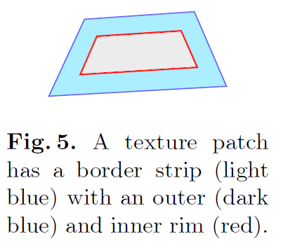
    • Poisson Editing
      • Have a look at UCAS.IO/Possion-Image-Edit
      • seams adjustment

        • perform local Poisson image editing[9, 16]

        • Poisson editing of a patch to a 20 pixel wide border strip[this]

        • 

  • Evaluation
    • Data Term and Photo-Consistency Check
      • 
      • 
    • Smoothness Term
      • 
    • Color Adjustment
      • 
      • 

Reference

1. 
2. 
3. 
4. 
5. 
6. 
7. 
8. 
9. 
10. 
11. 
12. 
13. 
14. 
15. 
16. 
17. 
18. 
19. 
20. 
21. 
22. 
23.